

Recipes: on price
Five scripts on candles alone - an EMA ribbon, volatility bands with squeezes, an anchored VWAP, session boxes and a higher-timeframe filter.
These recipes read only the bars themselves (open, high, low, close, volume and time), so they work on every market, every exchange and every plan. Each one is a whole script: copy it, or press Open in editor, and it runs as it is.
| Recipe | What it does | What it teaches |
|---|---|---|
| EMA ribbon with a trend tint | Four EMAs that turn green, red or gray by how they are stacked | ta.ema, conditional colors, fill between plots |
| Volatility bands and squeezes | ATR bands around an EMA, shaded when the Bollinger Bands fit inside them | tuples from ta.bb, history with [1], alert.on |
| Anchored VWAP from a date | A volume-weighted average and its bands from a moment you pick | input.time, state sums, resetting on a condition |
| Session ranges | A growing box for the Asia, London and New York sessions | session strings, time() with a session, functions with their own state, boxes |
| Higher-timeframe trend filter | Signals on your chart, kept only when a higher timeframe agrees | request.tf, confirmed bars, a filtered alert |
#EMA ribbon with a trend tint
A ribbon shows at a glance whether the averages agree. When the fastest EMA is above the next, and so on down to the slowest, the trend is up and the ribbon turns green; the opposite order turns it red; anything else is gray.
Data: candles only. Plan: every plan.
#The script
//@chartscript 1
indicator("EMA ribbon, trend tint", { overlay: true })
const fastLen = input.int(8, "Fastest EMA", { minval: 2 })
const step = input.int(8, "Step between EMAs", { minval: 1 })

const e1 = ta.ema(close, fastLen)
const e2 = ta.ema(close, fastLen + step)
const e3 = ta.ema(close, fastLen + 2 * step)
const e4 = ta.ema(close, fastLen + 3 * step)

// green when the averages are stacked fastest-on-top, red when stacked the other way, gray otherwise
const stackedUp = e1 > e2 && e2 > e3 && e3 > e4
const stackedDown = e1 < e2 && e2 < e3 && e3 < e4
const tint = stackedUp ? color.up : stackedDown ? color.down : color.muted

const top = plot(e1, "EMA 1", tint, 2)
plot(e2, "EMA 2", color.new(tint, 30))
plot(e3, "EMA 3", color.new(tint, 50))
const bottom = plot(e4, "EMA 4", color.new(tint, 65))
fill(top, bottom, color.new(tint, 88), "Ribbon")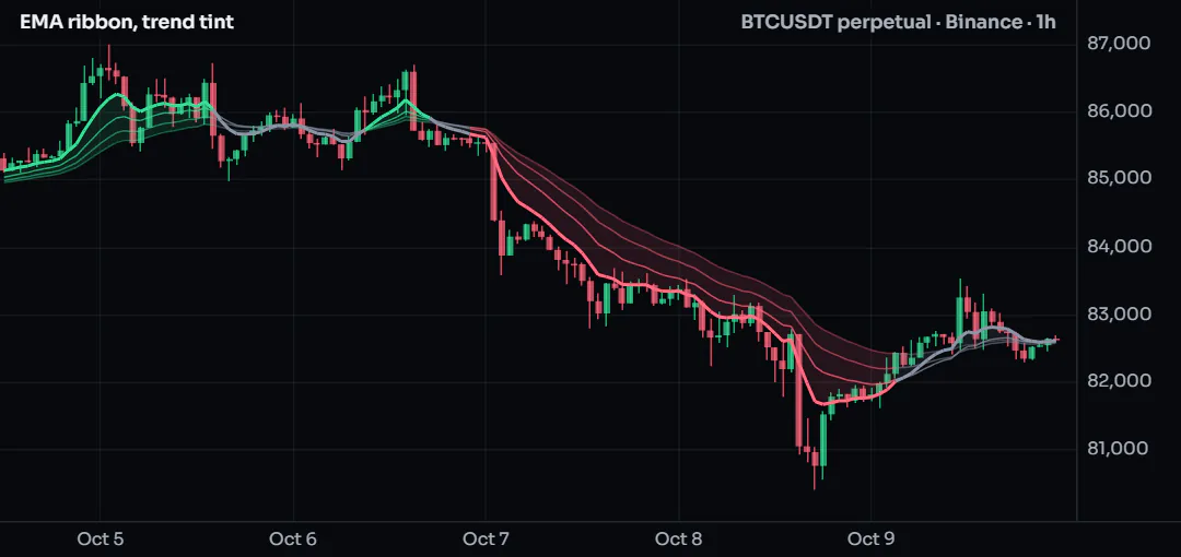
#How it works
- Two inputs set the fastest length and the step, so the four lengths are 8, 16, 24 and 32 by default.
stackedUpandstackedDowncompare neighbors only: if each EMA is above the next, the whole stack is in order.- One color,
tint, drives every line;color.new(tint, 30)makes the slower lines more transparent. plotreturns a handle;fill(top, bottom, ...)shades between the outer two.
#Customize it
- Use SMAs instead: replace
ta.emawithta.sma. - Make the gray state stand out less:
color.new(color.muted, 70)instead ofcolor.muted. - For a six-line ribbon, add
e5ande6and extend the two conditions.
#Run it
Add it to any chart. On a 1-hour chart the default 8-to-32 ribbon follows swings of a day or two; on a daily chart try a step of 20. The longer ribbon tutorial builds a five-line version step by step.
#Concepts used
ta.ema, conditional colors, fill, inputs.
#Volatility bands and squeezes
Volatility comes in waves. When the Bollinger Bands (based on the standard deviation) fit inside ATR bands (based on the average range), the market is unusually quiet, and quiet often comes before a move. This script draws the ATR bands, shades them while the squeeze is on, and has an alert for the moment it ends.
Data: candles only. Plan: every plan.
#The script
//@chartscript 1
indicator("Volatility bands and squeezes", { overlay: true })
const len = input.int(20, "Length", { minval: 2 })
const atrMult = input.float(1.5, "ATR bands, x ATR", { minval: 0.1, step: 0.1 })
const bbMult = input.float(2.0, "Bollinger Bands, x deviation", { minval: 0.1, step: 0.1 })

const mid = ta.ema(close, len)
const atr = ta.atr(len)
const upper = mid + atrMult * atr
const lower = mid - atrMult * atr
const [bbMid, bbUpper, bbLower] = ta.bb(close, len, bbMult)

// the squeeze: the deviation bands sit inside the range bands
const squeeze = bbUpper < upper && bbLower > lower
const released = squeeze[1] && !squeeze

const pUp = plot(upper, "Upper band", color.muted)
const pLo = plot(lower, "Lower band", color.muted)
plot(mid, "Middle", color.accent)
fill(pUp, pLo, squeeze ? color.new(color.amber, 82) : color.new(color.accent, 94), "Band")
plotshape(released && close > mid, "Released upward", shape.triangleup, location.belowbar, color.up, { size: size.small })
plotshape(released && close < mid, "Released downward", shape.triangledown, location.abovebar, color.down, { size: size.small })

alert.on(released, "Squeeze released", "{{ticker}} {{interval}}: the volatility squeeze ended at {{close}}")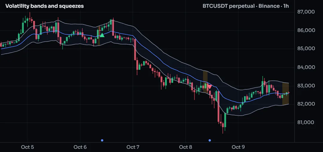
#How it works
ta.atr(len)is the average true range; the bands sitatrMultATRs either side of the EMA.ta.bbreturns three values at once (middle, upper, lower), unpacked withconst [a, b, c] = ....squeeze[1]is the previous bar's value of the condition, soreleasedis true on the first bar after a squeeze.- The fill's color can change from bar to bar: amber while squeezed, faint otherwise.
alert.ondeclares a condition; you turn it into a real alert from Create alert.
#Customize it
- A tighter definition of quiet: lower
atrMultto1.2; fewer, stronger squeezes. - Show the Bollinger Bands too:
plot(bbUpper, "BB upper", color.new(color.violet, 40))and the same forbbLower. - Count how long the squeeze lasted with a
statecounter and print it in a label when it ends.
#Run it
Any market, any timeframe. Squeezes are easiest to see on 15-minute to 4-hour charts. The direction marks only say on which side of the middle the bar closed; they are not a forecast.
#Concepts used
Tuples, history with [n], fill, alert.on.
#Anchored VWAP from a date
A VWAP answers "what is the average price paid, weighted by volume, since a moment that matters": a breakout, a news event, the start of a month. You pick that moment in the settings; the script sums price times volume from there and draws the average with one- and two-deviation bands.
Data: candles only (the chart's own volume). Plan: every plan.
#The script
//@chartscript 1
indicator("Anchored VWAP", { overlay: true })
const anchorTime = input.time(timestamp(2026, 10, 1), "Anchor (UTC)")
const showBands = input.bool(true, "Show the deviation bands")

// the first bar at or after the anchor starts the sums again
const started = time >= anchorTime
const startBar = started && (na(time[1]) || time[1] < anchorTime)

state sumPV = 0.0
state sumV = 0.0
state sumP2V = 0.0
if (startBar) {
    sumPV = 0
    sumV = 0
    sumP2V = 0
}
if (started && !na(volume)) {
    sumPV += hlc3 * volume
    sumV += volume
    sumP2V += hlc3 * hlc3 * volume
}

const vwap = started && sumV > 0 ? sumPV / sumV : na
const dev = started && sumV > 0 ? math.sqrt(math.max(0, sumP2V / sumV - vwap * vwap)) : na

plot(vwap, "Anchored VWAP", color.orange, 2)
plot(showBands ? vwap + dev : na, "+1 deviation", color.new(color.orange, 50))
plot(showBands ? vwap - dev : na, "-1 deviation", color.new(color.orange, 50))
plot(showBands ? vwap + 2 * dev : na, "+2 deviations", color.new(color.orange, 75))
plot(showBands ? vwap - 2 * dev : na, "-2 deviations", color.new(color.orange, 75))
plotshape(startBar, "Anchor", shape.diamond, location.belowbar, color.orange, { size: size.tiny })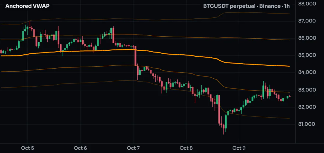
#How it works
input.timegives a date-and-time setting, in milliseconds UTC, the same unit astime.startBaris true on exactly one bar: the first whose time is at or after the anchor.- Three
statesums keep their values from bar to bar;startBarsets them back to zero. - The deviation is the volume-weighted standard deviation: the square root of the average of price squared minus the average squared.
- Before the anchor
vwapisna, so nothing is drawn there.
#Customize it
- Anchor on the start of each week instead of a date: replace
startBarwithtimeframe.change("1W")andstartedwithtrue. - Use the close instead of
hlc3as the price. - Pick the anchor from a list of events by adding several
input.timesettings and one VWAP per anchor (wrap the sums in a function: each call keeps its own state).
#Run it
Open the settings and set the anchor inside the bars on your chart. If the anchor is earlier than the oldest bar, the VWAP starts on the first bar; if it is in the future, nothing is drawn. Volume is each exchange's own, so two venues give slightly different lines.
#Concepts used
state, inputs, bars and time, na.
#Session ranges
Crypto trades around the clock, but the hours when Asia, London and New York are at their desks still have their own character. This script draws one box per session that grows with the session's high and low, then stays on the chart as a reference.
Data: candles only. Plan: every plan. Works on intraday charts (a daily bar covers every session at once).
#The script
//@chartscript 1
indicator("Session ranges", { overlay: true, max_boxes_count: 300 })
const asia = input.session("0000-0800", "Asia (UTC)")
const london = input.session("0700-1600", "London (UTC)")
const newYork = input.session("1330-2000", "New York (UTC)")
const showNames = input.bool(true, "Write the session name in each box")

// one session: a box that starts on its first bar and grows while the session is open
function sessionBox(sess, name, col) {
    const inSession = !na(time(timeframe.period, sess))
    state b: box = na
    state hi: float = na
    state lo: float = na
    if (inSession && (!inSession[1] || na(b))) {
        hi = high
        lo = low
        b = box.new(time, high, time_close, low, { xloc: xloc.bar_time, border_color: color.new(col, 40), bgcolor: color.new(col, 90),
            text: showNames ? name : "", text_color: col, text_size: size.small, text_halign: text.align_left, text_valign: text.align_top })
    } else if (inSession) {
        hi = math.max(hi, high)
        lo = math.min(lo, low)
        b.set_top(hi)
        b.set_bottom(lo)
        b.set_right(time_close)
    }
    return inSession
}

const inAsia = sessionBox(asia, "Asia", color.violet)
const inLondon = sessionBox(london, "London", color.accent)
const inNewYork = sessionBox(newYork, "New York", color.orange)
plot(inAsia && inLondon ? 1 : 0, "Asia-London overlap", { display: display.data_window })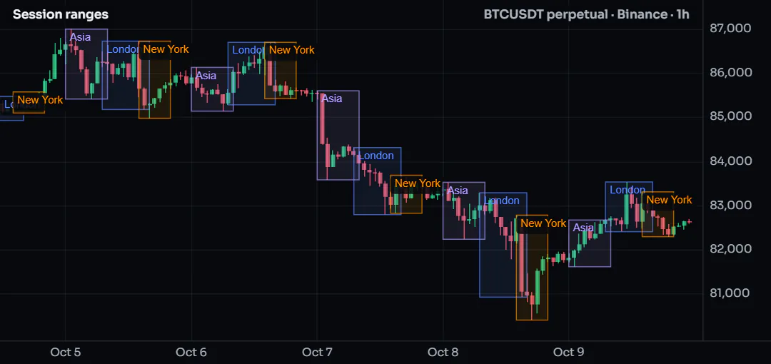
#How it works
- A session string is
"HHMM-HHMM"in UTC.time(timeframe.period, sess)is the bar's time inside the session andnaoutside it, so!na(...)tests "is this bar in the session". sessionBoxis called three times. Each call has its ownstatevariables, so the three boxes never mix.- On a session's first bar the function creates a box with
xloc.bar_time(left and right are times); on the next bars it moves the top, bottom and right edge. - The function returns whether the bar is in the session, so the script can use it afterwards (here, an overlap flag in the Data Window).
#Customize it
- Add a fourth session: one more
input.sessionand one moresessionBoxline. - Draw only the outline:
bgcolor: color.new(col, 100). - Mark breaks of the last session's range with
plotshape(close > ...); the session high and low tutorial shows how to keep the finished levels.
#Run it
Add it to a 5-minute to 1-hour chart. Session times are UTC; a timezone such as "America/New_York" can be given to time() as a third argument to follow daylight saving. The box limit is max_boxes_count; the oldest boxes go first.
#Concepts used
Sessions, functions and per-call state, drawings.
#Higher-timeframe trend filter
A signal on a 15-minute chart is more convincing when the 4-hour trend points the same way. This script reads a 4-hour EMA, draws it on your chart, and keeps a simple crossover signal only when the higher timeframe agrees, on closed bars only so the marks never change after the fact.
Data: candles of the same market at another timeframe. Plan: every plan (each requested timeframe counts toward your plan's request contexts, see Limits).
#The script
//@chartscript 1
indicator("Higher-timeframe trend filter", { overlay: true })
const htf = input.timeframe("240", "Trend timeframe")
const htfLen = input.int(50, "Trend EMA length", { minval: 2 })
const fastLen = input.int(9, "Signal EMA on this chart", { minval: 2 })

// both values from the higher timeframe's CLOSED bars (the default at: request.close never repaints)
const [htfEma, htfClose] = request.tf(htf, [ta.ema(close, htfLen), close])
const trendUp = htfClose > htfEma
const trendDown = htfClose < htfEma

const fast = ta.ema(close, fastLen)
const longSignal = barstate.isconfirmed && ta.crossover(close, fast) && trendUp
const shortSignal = barstate.isconfirmed && ta.crossunder(close, fast) && trendDown

plot(htfEma, "Higher-timeframe EMA", trendUp ? color.up : trendDown ? color.down : color.muted, 2, plot.style_stepline)
plot(fast, "Signal EMA", color.new(color.accent, 40))
plotshape(longSignal, "Long with the trend", shape.triangleup, location.belowbar, color.up, { size: size.small })
plotshape(shortSignal, "Short with the trend", shape.triangledown, location.abovebar, color.down, { size: size.small })

alert.on(longSignal, "Long with the trend", "{{ticker}} {{interval}}: crossed up with the higher timeframe trend at {{close}}")
alert.on(shortSignal, "Short with the trend", "{{ticker}} {{interval}}: crossed down with the higher timeframe trend at {{close}}")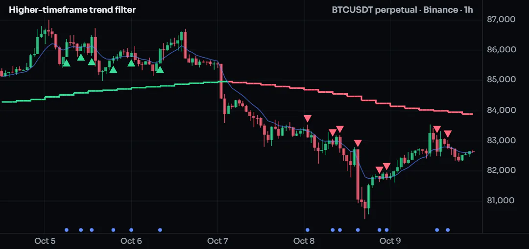
#How it works
request.tf(htf, [a, b])evaluates both expressions on the higher timeframe and returns them together; one request, one context.- With the default
at: request.closeeach chart bar sees the last closed higher bar, so history and live behave the same. barstate.isconfirmedkeeps the signal for the bar's close: a mark never appears and then vanishes.- The step-line style shows that the higher value only changes when a higher bar closes.
#Customize it
- Trend by slope instead of position:
const trendUp = htfEma > htfEma[1]inside the request:request.tf(htf, ta.ema(close, htfLen) > ta.ema(close, htfLen)[1]). - Use the daily trend: set the timeframe to
1D. - Replace the crossover with any signal of your own; keep the
&& trendUpfilter.
#Run it
Use a chart timeframe lower than the trend timeframe (a 15-minute chart with the 4-hour trend, for example). On a chart that is already at or above the trend timeframe the filter reads the chart's own bars. The multi-timeframe tutorial explains the at modes in detail.